Computing Ornstein-Uhlenbeck Process Trajectories in R

Compared to the Ruby version, computing this in R is much easier due to the built-in stochastic differential equation simulator. Assuming you have R installed, make sure you also install the sde package. Here is all the initial work that cleans up everything from your workspace, sets the initial value of the process, the end-point, how granular you want the simulation to be, and how many trajectories you want.

rm(list = ls(all = TRUE))
x0 = 50
end_point = 200
discretization_factor = 100
total_steps = end_point * discretization_factor
#Use the same seed for multiple trajectories if (number_trajectories > 1)
number_trajectories = 1
set.seed(rnorm(1))

Here we have a 0 drift parameter and a standard deviation of 1, followed by the simulation and plot of the process.

d = expression(0 * x)
s = expression(1)
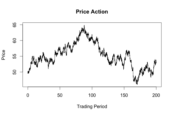
X = sde.sim(M=number_trajectories, X0=x0, T=end_point, N=total_steps, drift=d, sigma=s) plot(X,main="Price Action", xlab="Trading Period", ylab="Price")

Here is an image of one of the trajectories created by the code.

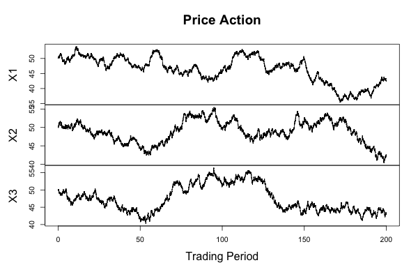
Making the small change in the code and switching number_trajectories = 1 to number_trajectories = 3 causes the simulator to produce a very convenient plot with all three trajectories. You could do some averaging or filtering with them if you wanted to. Below is an image of three trajectories.

As you can see, doing such simulations with R is very quick and easy. In fact, I think I may displace Ruby as my default language for such tasks.